Training in dStudio

Setting up the training

In this section of the tutorial you will use the Data Snapshot of the annotated images to create a Project in order to train an object detection or instance segmentation network in dStudio.

Since the Data Snapshot was already selected in the previous step, step two in the Projects workflow is displayed.

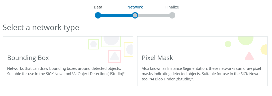
For this tutorial, select Bounding Box for object detection or Pixel Mask for instance segmentation, then click Next to proceed.

Important: Before making a selection, please take a moment to review which network is most suitable for your needs.

Which object finding network should I select?

Bounding Box vs. Pixel Mask

Aspect	Bounding Box (object detection)	Pixel Mask (instance segmentation)
Purpose	Identifies objects with rectangular bounding boxes around approximate locations.	Segments objects with pixel-level masks, delineating exact boundaries.
Performance	Priorities speed and efficiency, ideal for quick, real-time analysis.	Emphasises accuracy and detail, suited for in-depth processing.
Object overlap	The model might get confused when objects are very close together or on top of each other. This can make it hard to separate them correctly.	The model can clearly tell objects apart even when they overlap or are close together. This makes it useful in busy or crowded scenes.
Accuracy	Good for localisation but may include background in the box; less precise for irregular shapes.	High precision; captures exact object boundaries, ideal for overlapping or irregularly shaped objects.
Background noise handling	Draws a rectangle around an object, but it may include background clutter, which can lead to errors in identifying objects.	Precisely outlines an object's shape, ignoring background noise, making it more accurate in complex or crowded scenes.
Training complexity	Simpler to train, requiring less annotated data and computational resources.	More complex, demanding higher-quality annotations and greater computational power.
Best use cases	Counting & Sorting: Counting products on a conveyor belt. Presence/Absence check: Verifying a label is on a box. General location: Guiding a robot to a general pick-up zone.	Quality inspection: Finding cracks or scratches on a surface. Precise measurement: Measuring the area of a weld or sealant bead. Complex robotic gripping: Guiding a robot to a precise edge.
Core question	"Is the object there, and roughly where is it?"	"What is the object's exact shape, size, and condition?"
Target Nova tool	AI Object Detection (dStudio)	AI Blob Finder (dStudio)

How to choose?

Choose Bounding Box (object detection)

You should choose this option when your main goal is to simply find and count objects. The model will place a "Bounding Box" (a simple rectangle) around each item it finds.

Main Advantage: This method is fast and efficient. Because it only needs to find the coordinates of a box, it requires less computing power and is ideal for applications where speed is the top priority.

Main Limitation: You get no shape information. The box is just a rough location. This means you can't get precise measurements, and it can struggle to separate individual objects that are very close together or overlapping.

Choose Pixel Mask (instance segmentation):

You should choose this option when the object's exact shape and boundaries are critical. The model will create a "Pixel Mask" for every individual object it finds, even if they are in a jumbled pile.

Main Advantage: This method provides maximum detail and precision. You can measure the exact area of an object, identify objects with irregular shapes, and perfectly separate items that are overlapping.

Main Limitation: The primary consideration is the effort required to create your dataset. Drawing precise, "pixel-perfect" masks for every object is significantly more time-consuming.

ℹ️ This tutorial will continue with the object detection part. If you want to proceed with instance segmentation instead, the steps are the same.

As stated in the workflow, the following is important to consider when choosing the network model:

• Complex tasks often benefit from using a larger network, at the cost of increased inference times.
• Images will be scaled to the input resolution of the network. Tasks with many small details often benefit from using a network with a larger input resolution, but avoid input resolutions higher than your image resolution, since the upscaling can introduce artifacts.
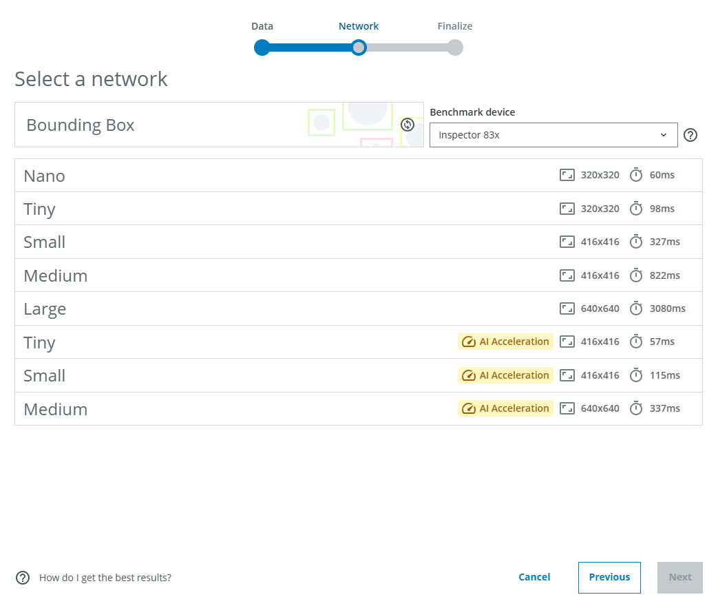
• If speed is important, consider AI acceleration. These networks trade some accuracy for much lower inference times, using dedicated hardware on the Inspector 83x/85x.

For each network model, the image input size to the network is displayed (eg. 320 pixels x 320 pixels for the Nano network). The estimated inference times are displayed on the right for each network model. The default shows the Benchmark average, but you can switch to the device you will use for inference.

For this tutorial, we will choose Medium without AI Acceleration. Then click Next. Note that augmentations are applied to the images during training, but currently these cannot be configured by the user.

Choose a Project name that makes it easy to remember which network model you have trained (you may end up training multiple networks). Click Create project.

Training progression

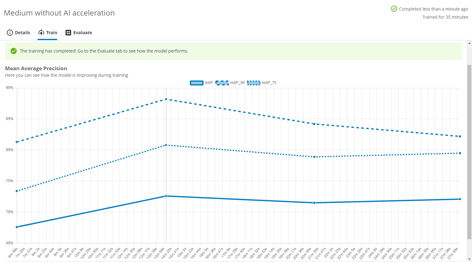
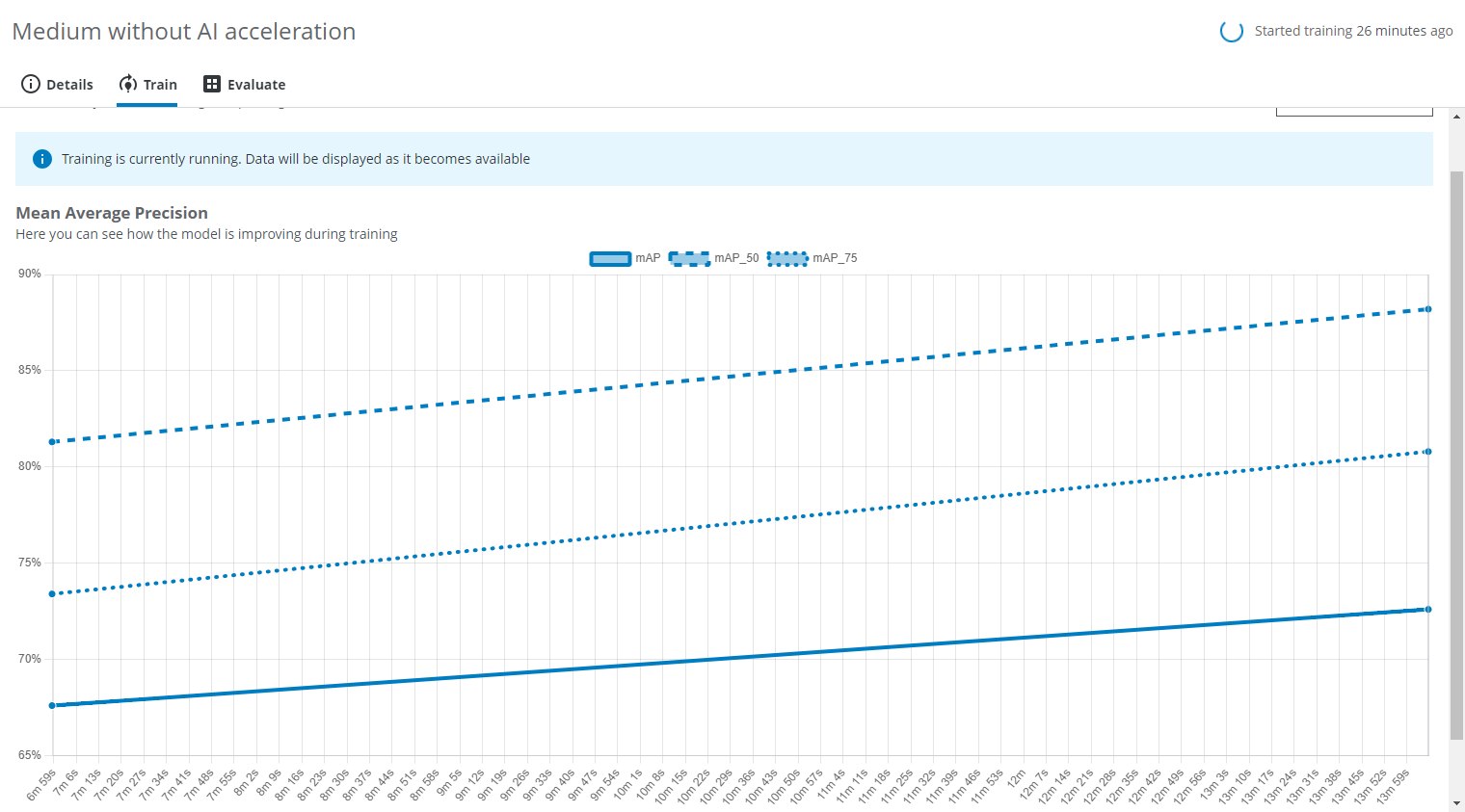
A training graph will become visible after a while in the Train tab. It shows how the Mean Average Precision improves during the training.

Advanced: Loss graph

Under Advanced you can find the Loss graph.

In the Details tab you can find the Domain name ("Glass vials") and the Data Snapshot name ("Green, clear, brown") in the Dataset field. You can also see the network model ("Medium 416x416") and the network type ("Object Detection").

Once the training is done, it will say so on the top right and inside the Train tab. Next, click on the Evaluate tab.